함수를 활용한 여러 변수 선택
- filter( ) : 메서드에서 변수 이름 패턴을 활용한 선택 (열 선택)
display(df_pr.filter(regex='se$') )
#위의 문장과 같은 역할을 한다
df_pr.loc[:,['Exercise']]

	Exercise
0	2
1	2
2	1
3	1
4	3
...	...
105	3
106	3
107	3
108	1
109	2
110 rows × 1 columns
regex : 정규표현식(regular expression), str(문자열)을 포함함
'^s' : 's'로 시작하는 이름/텍스트
's$' : 's'로 끝나는 이름/텍스트
- . dtypes: 변수형식 확인
df_ins.dtypes

age           int64
sex          object
bmi         float64
children      int64
smoker       object
region       object
charges     float64
dtype: object
int/float : 숫자
object : 문자열
변수 형식으로 선택
- include= ' 변수 형식' : '변수 형식'과 같은 변수를 선택함
- exclude= '변수 형식' : 변수 형식'과 같은 변수를 제외함
df_ins.select_dtypes(include='number')

	age	bmi	children	charges
0	19	27.900	0	16884.92400
1	18	33.770	1	1725.55230
2	28	33.000	3	4449.46200
3	33	22.705	0	21984.47061
4	32	28.880	0	3866.85520
...	...	...	...	...
1333	50	30.970	3	10600.54830
1334	18	31.920	0	2205.98080
1335	18	36.850	0	1629.83350
1336	21	25.800	0	2007.94500
1337	61	29.070	0	29141.36030
1338 rows × 4 columns
수치형(int, float) 변수
df_ins.select_dtypes(include='object')

	sex	smoker	region
0	female	yes	southwest
1	male	no	southeast
2	male	no	southeast
3	male	no	northwest
4	male	no	northwest
...	...	...	...
1333	male	no	northwest
1334	female	no	northeast
1335	female	no	southeast
1336	female	no	southwest
1337	female	yes	northwest
1338 rows × 3 columns
문자형(object) 변수
조건을 활용한 관측치 선택 :SQL에서 WHERE 절이나 Excel의 Filter와 같이 데이터에서 부분을 선택할 때 조건을 활용하는 경우 많음, [ ]나. loc [ ] 안에 조건식을 넣어서 조건과 일치하는 관측치만 선택 가능
- 1 단계 : 조건 설정(결과는 True/False) (bool 타입 Series)
- 2 단계 : [ ]와 조건을 활용한 관측치 선택
- 3 단계 : &와 |를 활용한 조건 결합( and -> & , or -> | ), 같은 인덱스끼리 연산함
# 1 단계
cond1 = df_ins['age'] < 30
# 2 단계
cond2 = df_ins['sex'] == 'female'
# 3 단계
cond = cond1 & cond2
df_ins[cond]

#위의 것과 같은 결과
df_ins[(df_ins['age'] < 30) & (df_ins['sex'] == 'female')]

#나이 30 미만 중 여성 선택
	age	sex	bmi	children	smoker	region	charges
0	19	female	27.900	0	yes	southwest	16884.92400
31	18	female	26.315	0	no	northeast	2198.18985
32	19	female	28.600	5	no	southwest	4687.79700
40	24	female	26.600	0	no	northeast	3046.06200
46	18	female	38.665	2	no	northeast	3393.35635
...	...	...	...	...	...	...	...
1328	23	female	24.225	2	no	northeast	22395.74424
1331	23	female	33.400	0	no	southwest	10795.93733
1334	18	female	31.920	0	no	northeast	2205.98080
1335	18	female	36.850	0	no	southeast	1629.83350
1336	21	female	25.800	0	no	southwest	2007.94500
201 rows × 7 columns- isin()을 활용한 특정 수준 관측치 선택
cond1 = df_ins['region'].isin(['southeast','northwest'])
# 위에 코드랑 같은 결과
(df_ins['region'] == 'southeast') | (df_ins['region'] == 'northwest')

0       False
1        True
2        True
3        True
4        True
        ...
1333     True
1334    False
1335     True
1336    False
1337     True
Name: region, Length: 1338, dtype: bool
isin() 뒤에 있는 게 있으면 True, 없으면 False(둘 중 하나만 있어도 True)
- Series의 between 메서드 : 특정 범위 내 관측치 선택 가능
# between(a>= n, b<=n)
cond1 = df_sp['math score'].between(80, 90, inclusive='left')

0      False
1      False
2      False
3      False
4      False
       ...
995     True
996    False
997    False
998    False
999    False
Name: math score, Length: 1000, dtype: bool
양쪽 끝 경계 포함 여부 지정 가능( 'both', 'left', 'right', 'neither')
bool Series(True/False) 앞에 ~ 를 붙여서 True와 False를 뒤집기 가능 (EX : ~cond1)
- . query() 메서드
df_sp.query('`math score`>= 90')90점 이상을 찾음
함수를 활용한 부분 관측치 선택
- head( )와 tail()
display("head()",df_ins.head())
display("tail()",df_ins.tail())

'head()'
age	sex	bmi	children	smoker	region	charges
0	19	female	27.900	0	yes	southwest	16884.92400
1	18	male	33.770	1	no	southeast	1725.55230
2	28	male	33.000	3	no	southeast	4449.46200
3	33	male	22.705	0	no	northwest	21984.47061
4	32	male	28.880	0	no	northwest	3866.85520

'tail()'
age	sex	bmi	children	smoker	region	charges
1333	50	male	30.97	3	no	northwest	10600.5483
1334	18	female	31.92	0	no	northeast	2205.9808
1335	18	female	36.85	0	no	southeast	1629.8335
1336	21	female	25.80	0	no	southwest	2007.9450
1337	61	female	29.07	0	yes	northwest	29141.3603
head() : 처음 n개의 행을 반환
tail() : 마지막 n개의 행을 반환
- sample( ) : 랜덤으로 추출
df_ins.sample(n=10)frac=0.005 : 비율로 추출 (EX: df_ins.sample(frac=0.005))
- nlargest( ), nsmallest( ) : 상위/하위 관측치 선택
df_ins.nlargest(10, 'charges')

	age	sex	bmi	children	smoker	region	charges
543	54	female	47.410	0	yes	southeast	63770.42801
1300	45	male	30.360	0	yes	southeast	62592.87309
1230	52	male	34.485	3	yes	northwest	60021.39897
577	31	female	38.095	1	yes	northeast	58571.07448
819	33	female	35.530	0	yes	northwest	55135.40209
1146	60	male	32.800	0	yes	southwest	52590.82939
34	28	male	36.400	1	yes	southwest	51194.55914
1241	64	male	36.960	2	yes	southeast	49577.66240
1062	59	male	41.140	1	yes	southeast	48970.24760
488	44	female	38.060	0	yes	southeast	48885.13561

df_ins.nsmallest(10, 'charges')

	age	sex	bmi	children	smoker	region	charges
940	18	male	23.21	0	no	southeast	1121.8739
808	18	male	30.14	0	no	southeast	1131.5066
1244	18	male	33.33	0	no	southeast	1135.9407
663	18	male	33.66	0	no	southeast	1136.3994
22	18	male	34.10	0	no	southeast	1137.0110
194	18	male	34.43	0	no	southeast	1137.4697
866	18	male	37.29	0	no	southeast	1141.4451
781	18	male	41.14	0	no	southeast	1146.7966
442	18	male	43.01	0	no	southeast	1149.3959
1317	18	male	53.13	0	no	southeast	1163.4627
nlargest(개수, 기준), nsmallest(개수, 기준)
중복값 제거
- drop_duplicates() : 중복값을 제거한 목록 생성 가능
df_ins.drop_duplicates(subset=['sex', 'region'])

	age	sex	bmi	children	smoker	region	charges
0	19	female	27.900	0	yes	southwest	16884.92400
1	18	male	33.770	1	no	southeast	1725.55230
2	28	male	33.000	3	no	southeast	4449.46200
3	33	male	22.705	0	no	northwest	21984.47061
4	32	male	28.880	0	no	northwest	3866.85520
...	...	...	...	...	...	...	...
1333	50	male	30.970	3	no	northwest	10600.54830
1334	18	female	31.920	0	no	northeast	2205.98080
1335	18	female	36.850	0	no	southeast	1629.83350
1336	21	female	25.800	0	no	southwest	2007.94500
1337	61	female	29.070	0	yes	northwest	29141.36030
1337 rows × 7 columns
subset을 기준으로 중복된 것을 없앰
관측치 정렬
- sort_values() : 관측치를 정렬
df_ins.sort_values(['age', 'charges'], ascending=[True, False])

	age	sex	bmi	children	smoker	region	charges
803	18	female	42.240	0	yes	southeast	38792.68560
759	18	male	38.170	0	yes	southeast	36307.79830
161	18	female	36.850	0	yes	southeast	36149.48350
623	18	male	33.535	0	yes	northeast	34617.84065
57	18	male	31.680	2	yes	southeast	34303.16720
...	...	...	...	...	...	...	...
768	64	female	39.700	0	no	southwest	14319.03100
801	64	female	35.970	0	no	southeast	14313.84630
752	64	male	37.905	0	no	northwest	14210.53595
534	64	male	40.480	0	no	southeast	13831.11520
335	64	male	34.500	0	no	southwest	13822.80300
1338 rows × 7 columns
기본은 오름차순, age는 오름차순(ascending=True), charges는 내림차순(asending=False)
- index를 활용한 정렬
df_ins = df_ins.sort_index()
df_ins

	age	sex	bmi	children	smoker	region	charges
0	19	female	27.900	0	yes	southwest	16884.92400
1	18	male	33.770	1	no	southeast	1725.55230
2	28	male	33.000	3	no	southeast	4449.46200
3	33	male	22.705	0	no	northwest	21984.47061
4	32	male	28.880	0	no	northwest	3866.85520
...	...	...	...	...	...	...	...
1333	50	male	30.970	3	no	northwest	10600.54830
1334	18	female	31.920	0	no	northeast	2205.98080
1335	18	female	36.850	0	no	southeast	1629.83350
1336	21	female	25.800	0	no	southwest	2007.94500
1337	61	female	29.070	0	yes	northwest	29141.36030
1338 rows × 7 columns
데이터 집계와 데이터 처리
수치형 변수의 집계값과 히스토그램 : 하나의 수치형 변수로 합계, 평균과 같은 집계값을 계산할 수 있고 히스토그램으로 분포를 확인
- 수치형 변수의 집계값 계산
df_ins['charges'].mean()
13270.422265141257

df_ins['charges'].sum()
17755824.990759

df_ins['charges'].var(), df_ins['charges'].std()
(146652372.1528548, 12110.011236693994)

df_ins['charges'].median()
9382.033

df_ins['region'].count()
1338
mean( ) : 평균
sum() : 합계
var() , std() : 분산과 표준편차
median() : 중앙값
count() : 관측치 수
- 히스토그램 그리기
import matplotlib.pyplot as plt
import seaborn as sns
라이브러리 불러오기
df_ins['age'].plot(kind='hist')
plt.show()
DataFrame의 plot 메서드 활용
plt.show() : 최종 그래프 출력함수, 생략 가능
sns.histplot(data=df_ins, x='age')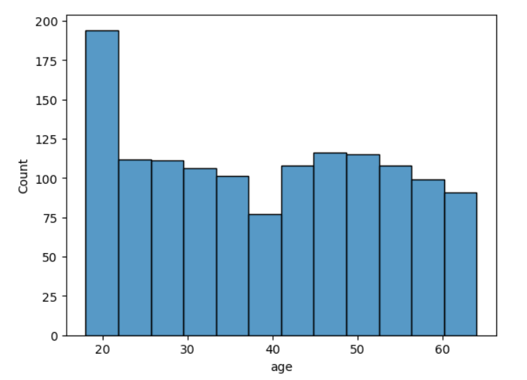
- 분위수 : 최솟값(minimum, 0%), Q1(1st Quartile, 25%), 중앙값(median, 50%), Q3(3rd Quartile, 75%), 최댓값(maximum, 100%)을 사분위수(quartile)이라고 부름
df_ins['charges'].quantile([0.0, 0.25, 0.5, 0.75, 1.0])

0.00     1121.873900
0.25     4740.287150
0.50     9382.033000
0.75    16639.912515
1.00    63770.428010
Name: charges, dtype: float64
quantile( ) : 계산할 분위(1.0이 최댓값)를 리스트로 묶기
- 상자그림(boxplot)
import seaborn as sns

# df_sp에서 'reading score'의 Q1(25%), 중위수(median, 50%), Q3(75%) 계산하기
print(df_sp['reading score'].quantile([0.25,0.5,0.75]))

# df_sp에서 'reading score'의 상자그림을 seaborn으로 그리기
display(" 'reading score'의 상자그림",sns.boxplot(data = df_sp,y = 'reading score'))

0.25    59.0
0.50    70.0
0.75    79.0
Name: reading score, dtype: float64
범주형 변수의 요약과 시각화
범주형 변수는 정해진 수준(level) 중에 하나의 값을 갖기 때문에 분석 방법이 단순하며 개수를 세면 됨
- 그룹별 건수 계산과 시각화 : 범주형 변수/그룹 변수로 수준별 관측치 수를 셀 수 있다.
df_ins['smoker'].value_counts()

smoker
no     1064
yes     274
Name: count, dtype: int64
value_counts() : 수준별 관측치 수 세기
sns.countplot(data=df_ins, x='smoker')
산점도와 상관계수의 활용
두 수치형 변수의 관계를 파악
- seaborn으로 산점도 그리기
mean_f = df_heights['father'].mean()
mean_s = df_heights['son'].mean()
print(mean_f, mean_s)

# plt.figure(figsize=(10,10))

plot_scatter = sns.scatterplot(data=df_heights, x='father', y='son', alpha=0.3)

# plot_scatter.axhline(mean_s) # 수평선 추가
# plot_scatter.axvline(mean_f) # 수직선 추가
df_heights[['father','son']].cov()
	father	son
father	48.608307	24.989192
son	24.989192	51.113092

df_heights[['father','son']].corr()
	father	son
father	1.000000	0.501338
son	0.501338	1.000000
공분산, 상관관계 계산 : 상관관계가 커질수록 연관성이 큼
그룹별 집계값의 계산과 분포 비교
범주형 변수를 그룹처럼 활용해서 그룹별 평균을 계산하고, 그룹별 상자그림을 그려서 그룹 간 분포를 비교
한 변수의 집계에서 groupby()를 추가하면 되고, 필요에 따라 agg()를 활용 가능
1. 그룹을 나눔
2. 변수 선택
3. 집계 선택
- 그룹별 평균 계산(DataFrame 형식으로 출력)
df_ins.groupby(['sex','smoker'], as_index=False)['charges'].agg(['min','max','mean'])

	sex	smoker	min	max	mean
0	female	no	1607.5101	36910.60803	8762.297300
1	female	yes	13844.5060	63770.42801	30678.996276
2	male	no	1121.8739	32108.66282	8087.204731
3	male	yes	12829.4551	62592.87309	33042.005975
groupby() : 그룹별 평균 계산(여러 개의 그룹 변수 가능)
as_index= : 데이터 프레임으로 변경, (기본은 True(시리즈로 출력))
agg() : 여러 집계값 계산
[실습] 변수 관계 탐색
1. 데이터 df_sp에서 범주형 변수(열) 하나를 선택해서 그룹을 나눈 후 수치형 변수(열) 하나를 선택하여 평균을 계산 및 상자그림 그리기
2. 데이터 df_sp에서 임의의 두 범주형 변수(열)를 선택하여 math score의 평균을 계산하기
3. 의 세 변수를 x, y, hue로 활용해 seaborn으로 상자그림 그리기
# 1. 데이터 df_sp에서 범주형 변수(열) 하나를 선택해서 그룹을 나눈 후 수치형 변수(열) 하나를 선택하여 평균을 계산 및 상자그림 그리기
# 범주형 gender, 수치형 math score
display(df_sp.groupby('gender', as_index=False)['math score'].mean())
sns.boxplot(data = df_sp, x ='gender',y ='math score')

	gender	math score
0	female	63.633205
1	male	68.728216
# 2. 데이터 df_sp에서 임의의 두 범주형 변수(열)를 선택하여 math score의 평균을 계산하기
df_sp.groupby(['gender','race/ethnicity'],as_index=False)['math score'].mean()

	gender	race/ethnicity	math score
0	female	group A	58.527778
1	female	group B	61.403846
2	female	group C	62.033333
3	female	group D	65.248062
4	female	group E	70.811594
5	male	group A	63.735849
6	male	group B	65.930233
7	male	group C	67.611511
8	male	group D	69.413534
9	male	group E	76.746479
# 3.의 세 변수를 x, y, hue로 활용해 seaborn으로 상자그림 그리기
sns.boxplot(data = df_sp , x= 'race/ethnicity',y='math score',hue='gender')
'ABC 부트캠프 데이터 탐험가 4기' 카테고리의 다른 글
| [10 일차] ABC 부트캠프 : 데이터 전처리 예제 (0) | 2024.07.17 |
|---|---|
| [9 일차] ABC 부트캠프 : 데이터 집계와 시각화(1) (0) | 2024.07.16 |
| [7일차] ABC 부트캠프 : pandas 기초 , 데이터 전처리 기초(1) (0) | 2024.07.14 |
| [6일차] ABC 부트캠프 : Jupyter Notebook 활용 및 Python 기초 (4) (0) | 2024.07.12 |
| [5일차] ABC 부트캠프 : Jupyter Notebook 활용 및 Python 기초 (3) (0) | 2024.07.11 |